TL;DR. Reinforcement learning (RL) recipes for vision-language-action (VLA) models update one decision variable: the action. A world-action model (WAM) has two — the action chunk and the imagined future. We argue that action-only RL leaves the world branch task-blind, and propose dual-branch RL, a PPO-style objective in which the video branch is also made accountable for task return. On LIBERO-Long with Fast-WAM as the base policy, dual-branch RL lifts the success rate from $91.1\%$ to $\mathbf{96.0}\%$ in 1k steps, versus $94.5\%$ for action-only Flow-SDE.
1. Introduction
From VLA to RL post-training. Vision-language-action models have become the dominant recipe for generalist robot policies. RT-2 [1] casts robot actions as text tokens and co-fine-tunes a vision-language model on web and robot data; OpenVLA [2] provides an open 7B discrete-action instantiation; $\pi_0$ [3] replaces action tokens with a flow-matching action expert, yielding continuous action chunks with high-frequency control. Imitation learning alone, however, is bounded by demonstration coverage. This has motivated a wave of RL post-training methods that convert a supervised VLA into a return-maximizing policy: SimpleVLA-RL [4] scales online RL for discrete-action VLAs, while $\pi$RL [5] targets flow-based VLAs with two flow-compatible estimators — Flow-Noise, which treats denoising as a discrete-time MDP with a learnable noise network for exact log-likelihoods, and Flow-SDE, which couples a denoising MDP with the environment MDP through an ODE-to-SDE conversion.
World-action models. In parallel, world-action models (WAMs) [6] have emerged as a response to the supervision deficit of pure VLA training: instead of predicting actions alone, the model also predicts how the visual world evolves, and the predicted future is made action-facing [6]. A representative instantiation is Fast-WAM [7], a mixture-of-transformers (MoT) that couples a video diffusion transformer with an action expert under shared attention, and shows that video co-training is essential while test-time future imagination can largely be skipped.
The gap. RL methods for WAMs are, to date, inherited verbatim from the VLA literature: they apply a flow-compatible estimator such as Flow-SDE to the action branch only. We contend that this under-uses the architecture. In Fast-WAM, action tokens are not allowed to attend to future video tokens, and the clean first-frame latent is the only shared anchor between the two branches [7]. Consequently the world branch can influence control only through the shared representation — and under action-only RL that representation receives no gradient from the task return. The video branch keeps minimizing a flow-matching reconstruction loss that is indifferent to whether the imagined future corresponds to a successful grasp or a dropped object. The capacity spent on future prediction is, in control terms, never credited.
Our approach. We propose dual-branch RL: both branches of a WAM are treated as stochastic policies over their own decision variables and are updated with a shared advantage estimate. Concretely,
- Action branch. We adopt Flow-SDE [5] and derive a closed-form per-step Gaussian importance ratio, so the likelihood of the whole denoising chain is available without numerical integration (Sec. 3.2).
- Video branch. Following the treatment of continuous latent tokens in LaST-R1 [8], we model the video latent as an isotropic Gaussian centered at the current policy output and obtain a lightweight step-level ratio over subsampled latent tokens (Sec. 3.3).
- Mixed ODE–SDE rollout. Integrating likelihoods over the entire video denoising chain is prohibitive. We therefore randomize a single denoising index per rollout and compute the video-branch RL loss only there, keeping memory and compute close to a pure-ODE rollout (Sec. 3.4).
On LIBERO-Long, starting from the same Fast-WAM checkpoint, dual-branch RL reaches $96.0\%$ success after 1k RL steps versus $94.5\%$ for action-only Flow-SDE — a $+1.5$ point margin that opens up early and persists.
2. Preliminaries
2.1 Flow-based action generation
Let $\mathbf{a}_t \in \mathbb{R}^{H \times d}$ denote an action chunk of horizon $H$ predicted at environment step $t$, and let $\tau \in [0, 1]$ be the continuous flow time. Conditional flow matching [9, 10] defines a probability path from noise to data by linear interpolation,
\[\mathbf{a}_t^{\tau} = \tau \, \mathbf{a}_t + (1 - \tau) \, \boldsymbol{\epsilon}, \qquad \boldsymbol{\epsilon} \sim \mathcal{N}(\mathbf{0}, \mathbf{I}),\]and regresses a velocity field $\mathbf{v}\theta(\mathbf{a}_t^{\tau}, \tau, \mathbf{c}_t)$ toward $\dot{\mathbf{a}}_t^{\tau} = \mathbf{a}_t - \boldsymbol{\epsilon}$, where $\mathbf{c}_t$ is the shared observation–language context. Sampling integrates the ODE $\mathrm{d}\mathbf{a}^{\tau} = \mathbf{v}\theta \, \mathrm{d}\tau$ from $\tau = 0$ to $\tau = 1$. Under this parameterization the one-step estimate of the clean action is
\[\hat{\mathbf{a}}_t^{\tau} = \mathbf{a}_t^{\tau} + (1 - \tau) \, \mathbf{v}_\theta(\mathbf{a}_t^{\tau}, \tau, \mathbf{c}_t).\]Because sampling is deterministic, a pure-ODE policy has no tractable, non-degenerate action likelihood — which is precisely why RL on flow policies requires an explicit change of measure [5].
2.2 World-action models
A WAM augments the action expert with a world branch that predicts future visual latents $\mathbf{Z}t = (\mathbf{z}{t,1}, \dots, \mathbf{z}_{t,N})$ of the next $T$ frames. Fast-WAM [7] implements this as an MoT over a pretrained video DiT and a lightweight action DiT, partitioning tokens into (i) clean latents of the first observation frame, which act as the shared visual anchor, (ii) noisy latents of future frames, used only during training, and (iii) action tokens. The attention mask is deliberately asymmetric: future video tokens are invisible to action tokens, and first-frame tokens attend to nothing. Training minimizes
\[\mathcal{L}_{\text{SFT}} = \underbrace{\mathcal{L}_{\text{FM}}(\mathbf{a}_{1:H})}_{\text{action branch}} \;+\; \lambda \underbrace{\mathcal{L}_{\text{FM}}(\mathbf{Z}_{1:T})}_{\text{video branch}} .\]Two properties of this design motivate our method. First, the video branch is load-bearing: removing video co-training degrades performance far more than removing test-time imagination [7]. Second, the branch is architecturally decoupled at inference: with action tokens masked from future video tokens, the only channel through which world modeling can shape control is the shared representation. Dual-branch RL is designed to make that channel carry return information.
3. Dual-Branch RL
3.1 A shared-advantage objective over two branches
Let $\mathbf{a}_t$ be the action chunk and $\mathbf{Z}_t$ the future latent produced at environment step $t$. We write the WAM policy as a product over branches conditioned on the shared context $\mathbf{c}_t$,
\[\pi_\theta(\mathbf{a}_t, \mathbf{Z}_t \mid \mathbf{c}_t) \;=\; \pi_\theta^{a}(\mathbf{a}_t \mid \mathbf{c}_t) \; \pi_\theta^{z}(\mathbf{Z}_t \mid \mathbf{c}_t), \tag{1}\]i.e. we treat the branches as conditionally independent given $\mathbf{c}_t$. This is an approximation — the two branches interact through shared attention — but it is the same factorization adopted by LAPO in LaST-R1 [8] for jointly optimizing latent reasoning and action generation, and it keeps each ratio computable in closed form.
Both branches are then updated with the same advantage estimate $\hat{A}_t$ (GAE [11]) computed from the environment return:
\[\mathcal{L}_{\text{policy}}(\theta) = -\,\mathbb{E}_t \Bigg[ \sum_{k \in \{a, z\}} \min\Big( r_t^{k}(\theta) \, \hat{A}_t ,\; \operatorname{clip}\big( r_t^{k}(\theta),\, 1 - \epsilon_{\min},\, 1 + \epsilon_{\max} \big) \, \hat{A}_t \Big) \Bigg]. \tag{2}\]Here $r_t^{k}(\theta) = \pi_\theta^{k}(\cdot \mid \mathbf{c}t) / \pi{\theta_{\text{old}}}^{k}(\cdot \mid \mathbf{c}t)$ is the per-branch importance ratio, and $(\epsilon{\min}, \epsilon_{\max})$ are asymmetric clip bounds: we follow LAPO [8] in decoupling the lower and upper range instead of using the symmetric range of vanilla PPO [12], which lets the update grow faster on positively advantaged samples while remaining conservative on negative ones. The ratio is evaluated on the stored rollout variables under both the current and the behavior policy. We omit the value-function and entropy terms for brevity; the full objective is $\mathcal{L} = \mathcal{L}{\text{policy}} + \lambda_v \mathcal{L}{\text{value}} + \lambda_{\text{SFT}} \mathcal{L}_{\text{SFT}}$.
Why share the advantage? $\hat{A}_t$ measures whether the executed action was better than expected. Feeding the same signal into the video branch is exactly the inductive bias we want: imagined futures that precede a high-return action are reinforced, futures that precede a failure are suppressed. The video branch stops being a passive reconstruction head and becomes an action-facing predictor in the sense of [6].
3.2 Action branch: Flow-SDE with a closed-form ratio
We convert the deterministic flow-matching ODE of Sec. 2.1 into a stochastic differential equation that preserves the marginal $q_\tau(\mathbf{a}^{\tau})$ [5]:
\[\mathrm{d}\mathbf{a}^{\tau} = \Big[ \underbrace{\mathbf{v}_\theta(\mathbf{a}^{\tau}, \tau, \mathbf{c}_t)}_{\text{velocity}} \;-\; \tfrac{1}{2}\sigma_\tau^{2} \underbrace{\nabla \log q_\tau(\mathbf{a}^{\tau})}_{\text{score}} \Big] \mathrm{d}\tau \;+\; \sigma_\tau \, \mathrm{d}\mathbf{w}_\tau . \tag{3}\]For the linear path of Sec. 2.1, the score admits the identity [5]
\[\nabla \log q_\tau(\mathbf{a}^{\tau}) = -\,\frac{\mathbf{a}^{\tau}}{\tau} - \frac{1 - \tau}{\tau}\,\mathbf{v}_\theta(\mathbf{a}^{\tau}, \tau, \mathbf{c}_t) = -\,\frac{\hat{\mathbf{a}}^{\tau}}{\tau}, \tag{4}\]using the one-step clean-action estimate of Sec. 2.1. Substituting Eq. (4) into Eq. (3) gives the compact drift used throughout this post:
\[\boxed{\; \mathrm{d}\mathbf{a}^{\tau} = \Big[ \mathbf{v}_\theta(\mathbf{a}^{\tau}, \tau, \mathbf{c}_t) + \frac{\sigma_\tau^{2}}{2\tau}\,\hat{\mathbf{a}}^{\tau} \Big] \mathrm{d}\tau + \sigma_\tau \, \mathrm{d}\mathbf{w}_\tau \;} \tag{5}\]Discretizing with step $\delta = 1/K$ and writing $\mathbf{u}\theta^{\tau} \triangleq \mathbf{v}\theta + \tfrac{\sigma_\tau^2}{2\tau}\hat{\mathbf{a}}^{\tau}$ for the drift, the transition is an isotropic Gaussian [5],
\[p_\theta\big(\mathbf{a}^{\tau + \delta} \mid \mathbf{a}^{\tau}\big) = \mathcal{N}(\boldsymbol{\mu}_\tau, \boldsymbol{\Sigma}_\tau), \qquad \begin{cases} \boldsymbol{\mu}_\tau = \mathbf{a}^{\tau} + \mathbf{u}_\theta^{\tau} \, \delta,\\[2pt] \boldsymbol{\Sigma}_\tau = \sigma_\tau^{2} \, \delta \, \mathbf{I}. \end{cases} \tag{6}\]3.3 Video branch: latent tokens as Gaussian decision variables
The video branch emits a tensor of continuous latents rather than a categorical token, so no exact likelihood is available. Following LaST-R1 [8], we place an isotropic Gaussian of fixed width $\sigma_z$ around the deterministic output of the current policy and treat the latent tensor as the branch’s decision variable:
\[\pi_\theta^{z}(\mathbf{Z}_t \mid \mathbf{c}_t) \;\propto\; \exp\!\left( -\,\frac{1}{2\sigma_z^{2}} \sum_{i=1}^{N_z} \big\lVert \mathbf{z}_{t,i}^{\text{old}} - \mathbf{z}_{t,i}^{\theta} \big\rVert^{2} \right), \tag{8}\]where $\mathbf{z}{t,i}^{\text{old}}$ are the latents stored in the rollout buffer, $\mathbf{z}{t,i}^{\theta}$ the latents the current policy would produce for the same context, and $N_z$ the number of tokens retained after a downsampling.
When the branch is rolled out deterministically, the stored latents are the behavior policy’s output, $\mathbf{z}{t,i}^{\theta{\text{old}}} = \mathbf{z}_{t,i}^{\text{old}}$, the second term vanishes, and Eq. (9) reduces to the single-term form used in [8]:
\[r_t^{z}(\theta) = \frac{\pi_\theta(\mathbf{Z}_t^{\text{old}} \mid \cdot)}{\pi_{\theta_{\text{old}}}(\mathbf{Z}_t^{\text{old}} \mid \cdot)} = \exp\!\left( -\frac{1}{2\sigma_z^{2}} \sum_{i=1}^{N_z} \big\lVert \mathbf{z}_{t,i}^{\text{old}} - \mathbf{z}_{t,i}^{\theta} \big\rVert^{2} \right). \tag{10}\]3.4 Randomly choose steps
Making the video branch stochastic at every one of the $K$ denoising steps would require storing $K$ latent tensors per environment step and backpropagating a ratio through the full chain — prohibitive for a 5B-parameter video DiT. We instead adopt a Random Strategy: we draw a single index $n \sim \mathcal{U}{0, \dots, K-1}$, where pre-step latent feature noise is injected and the transition is recorded, and the video-branch ratio is computed at step $n$ only.
3.5 Algorithm
Algorithm 1  Dual-branch PPO for WAM policies (one iteration)
──────────────────────────────────────────────────────────────────────────────
Require: WAM policy π_θ = (action expert, video DiT), SFT weights θ, value net V_φ,
         denoising steps K, step δ = 1/K, schedule scales α_a, α_z,
         video-token subsample size N_z, clip bounds (ε_min, ε_max)

 1:  θ_old ← θ
 2:  ══════════ ROLLOUT  (behaviour policy θ_old, no gradients) ═════════════
 3:  for each environment step t do
 4:      c_t ← encode(o_{≤t}, ℓ)                              # shared context
 5:      n ∼ Uniform{0, …, K−1}                               # ONE index, both branches
 6:
 7:      # ── action branch: K steps, noise only at k = n ────────────────────
 8:      a^{τ_0} ∼ N(0, I)
 9:      for k = 0 … K−1 do
10:          τ_k ← k/K ;   v_k ← v^a_{θ_old}(a^{τ_k}, τ_k, c_t)
11:          â_k ← a^{τ_k} + (1 − τ_k) v_k                    # clean-action estimate
12:          u_k ← v_k + ((σ^a_{τ_k})² / (2 τ_k)) â_k         # score-corrected drift
13:          if k = n then   a^{τ_k+δ} ∼ N(a^{τ_k} + δ u_k , (σ^a_{τ_k})² δ I)
14:          else            a^{τ_k+δ} ← a^{τ_k} + δ u_k      # deterministic ODE step
15:      end for
16:      store (a^{τ_n}, Δa ← a^{τ_n+δ} − a^{τ_n}, u_n)       # ONE transition only
17:
18:      # ── video branch: same K steps, noise at the SAME k = n ─────────────
19:      z^{τ_0} ∼ N(0, I)
20:      for k = 0 … K−1 do
21:          w_k ← v^z_{θ_old}(z^{τ_k}, τ_k, c_t)
22:          ẑ_k ← z^{τ_k} + (1 − τ_k) w_k
23:          m_k ← w_k + ((σ^z_{τ_k})² / (2 τ_k)) ẑ_k
24:          if k = n then   z^{τ_k+δ} ∼ N(z^{τ_k} + δ m_k , (σ^z_{τ_k})² δ I)
25:          else            z^{τ_k+δ} ← z^{τ_k} + δ m_k
26:      end for
27:      store (z^{τ_n}, Δz ← z^{τ_n+δ} − z^{τ_n}, m_n)       # subsampled to N_z tokens
28:
29:      execute the first h actions of a^{τ_K} = a¹;  observe r_t and o_{t+1}
30:  end for
31:
32:  ══════════ UPDATE ══════════════════════════════════════════════════════
33:  Â_t ← GAE(r_{1:T}, V_φ)                                   # one shared advantage
34:  for each PPO epoch do
35:      for each minibatch do
36:          # re-evaluate ONE denoising step per branch, at the STORED states
37:          u^θ_n ← drift of v^a_θ at (a^{τ_n}, τ_n, c_t)     #   1 forward pass
38:          m^θ_n ← drift of v^z_θ at (z^{τ_n}, τ_n, c_t)     #   1 forward pass
39:          log r^a ← Eq. (7) with (Δa, u^θ_n, u_n)
40:          log r^z ← Eq. (7) with (Δz, m^θ_n, m_n)          # over subsampled tokens
41:          update θ with Eq. (2) ;  update φ with the value loss
42:      end for
43:  end for
3.6 Notation
| Symbol | Meaning |
|---|---|
| $t$ | environment time step |
| $\tau \in [0,1]$ | flow-matching time; $\tau = 1$ is data |
| $K = 10$, $\delta = 1/K = 0.1$ | number of denoising steps, integration step size |
| $\mathbf{c}_t$ | shared observation–language context |
| $\mathbf{a}_t^{\tau}, \mathbf{a}_t$ | noisy action chunk at flow time $\tau$; clean action chunk |
| $\mathbf{v}_\theta(\cdot)$ | predicted velocity field |
| $\hat{\mathbf{a}}^{\tau}$ | one-step clean-action estimate, Sec. 2.1 |
| $\sigma_\tau = \alpha\sqrt{\tau/(1-\tau)}$ | SDE noise schedule of the action branch |
| $\mathbf{Z}t, \mathbf{z}{t,i}$ | future video latents; the $i$-th latent token |
| $N_z$ | number of latent tokens retained after subsampling |
| $\sigma_z$ | fixed width of the Gaussian over video latents |
| $r_t^{a}, r_t^{z}$ | importance ratio of the action / video branch |
| $\hat{A}_t$ | (shared) GAE advantage |
| $\epsilon_{\min}, \epsilon_{\max}$ | asymmetric PPO clip bounds |
Three notation traps are worth flagging, since all of them appear in the source draft: (i) $\sigma$ denotes different quantities in the two branches — a $\tau$-dependent SDE schedule in Eq. (5) and a fixed latent width in Eq. (10) — hence $\sigma_\tau$ versus $\sigma_z$; (ii) $A$ is used both for advantage and for action, hence advantage $\hat{A}t$ (decorated) versus action $\mathbf{a}$ (lowercase bold); (iii) $\delta = 0.1$ is the *integration step size* fixed by $K = 10$, not a noise level — the noise scales are $\sigma\tau$ and $\sigma_z$.
4. Experiments
4.1 Setup
Base policy. Fast-WAM [7], whose action branch is a flow-matching action expert and whose video branch is a video DiT; we RL-fine-tune from the supervised checkpoint without any additional embodied pretraining.
Benchmark. LIBERO [13], a lifelong manipulation benchmark with four task suites (Spatial, Object, Goal, Long). We report the LIBERO-Long suite, which has the longest horizons and is therefore the most sensitive to credit assignment over time. For reference, Fast-WAM reports $98.2 / 100.0 / 97.0 / 95.2$ (avg. $97.6\%$) on the four suites under its own full training recipe [7].
Training. PPO with the dual-branch objective of Eq. (2); global batch size 2048; noise scale $\sigma = 0.1$; 1k RL training steps; evaluation every 10 steps. Advantages are computed with GAE [11] from binary task-success returns. Infrastructure is built on RLinf [14].
Denoising budget. We set the number of flow-matching denoising steps to $K = 10$ (hence $\delta = 0.1$), whereas the LIBERO-Long numbers reported in [7] were obtained with $K = 20$. This is a deliberate trade-off: rollout dominates wall-clock time in on-policy RL, and halving $K$ roughly halves the cost of every action sampled on the robot side. The cost is discretization error, and it is visible in the starting point — our checkpoint evaluates to $91.1\%$ rather than the reported $95.2\%$. This $4.1$-point offset is a property of the shared starting checkpoint, so it applies identically to both curves in Fig. 1 and does not affect the comparison between them. We did not re-run the $K = 20$ configuration under our own protocol, so the residual part of the gap may also reflect the checkpoint itself, the evaluation protocol, or random seeds.
Baseline. The same Fast-WAM checkpoint fine-tuned with Flow-SDE [5] applied to the action branch only — i.e. Eq. (2) restricted to $k \in {a}$, with the same $K = 10$ rollout. This isolates the contribution of the video branch.
4.2 Results
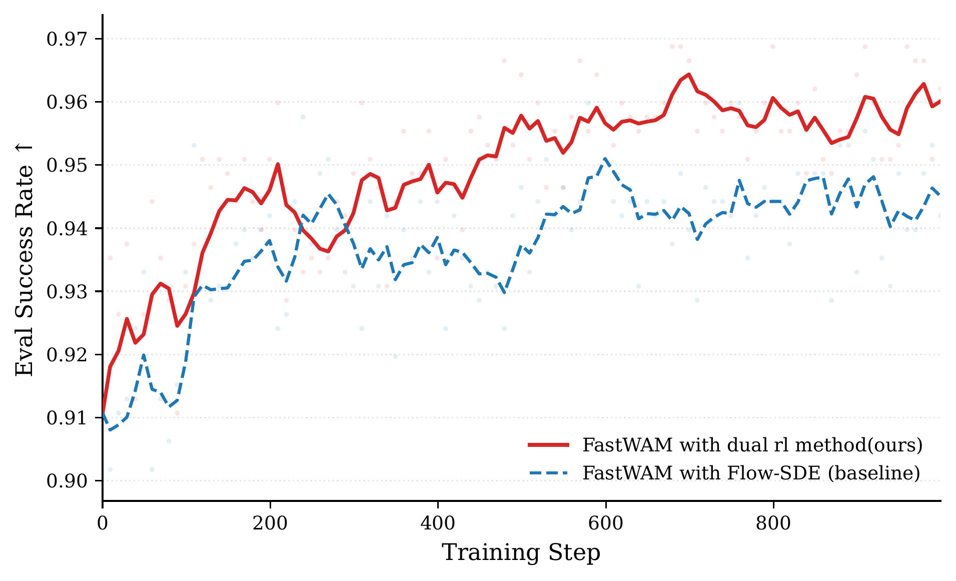
Figure 1. LIBERO-Long success rate versus RL training steps (mean over the evaluation set; one evaluation every 10 steps). Red: Fast-WAM + dual-branch RL (ours). Blue: Fast-WAM + Flow-SDE on the action branch only (baseline). Both runs start from the same supervised checkpoint ($91.1\%$).
| Method | $K$ | Init. | Final | Last-100 mean | Peak | $\Delta$ vs. baseline |
|---|---|---|---|---|---|---|
| Fast-WAM (SFT checkpoint, ours) | $10$ | $91.1\%$ | — | — | — | — |
| + Flow-SDE (action branch only) | $10$ | $91.1\%$ | $94.5\%$ | $94.4\%$ | $95.1\%$ | — |
| + Dual-branch RL (ours) | $10$ | $91.1\%$ | $\mathbf{96.0}\%$ | $\mathbf{96.0}\%$ | $\mathbf{96.5}\%$ | $\mathbf{+1.5}$ |
Table 1. LIBERO-Long success rate. “Final” is the last evaluation at step 1000; “last-100 mean” averages the final ten evaluations to remove evaluation noise. The last row is copied from [7] for reference only: it uses a different denoising budget and protocol, so it is not a like-for-like comparison with the three rows above it.
4.3 Analysis
The margin opens early and persists. The two curves separate within the first $\sim 200$ steps and the gap never closes; the peak-to-peak advantage reaches $2.6$ points and settles at $+1.5$ points. This is consistent with the intended mechanism: the video branch starts receiving return signal immediately, so the shared representation is reshaped from the beginning of RL rather than only through the action head.
A higher plateau, not just faster climbing. The baseline saturates around $94.5\%$ and its last-100 mean ($94.4\%$) is below its peak ($95.1\%$), i.e. it mildly over-optimizes and drifts back. Ours keeps improving and its last-100 mean matches its final value, suggesting that the latent-space trust region of Eq. (10) also acts as a stabilizer for the joint update.
RL repays the discretization error, and then some. Recall that we deliberately pay $4.1$ points up front by halving the denoising budget ($95.2\% \to 91.1\%$). After 1k RL steps, ours reaches $96.0\%$ at $K = 10$ — above the $95.2\%$ that [7] reports at $K = 20$, using half the sampling compute per action. In other words, RL does not merely close the gap that coarse sampling opened; it more than covers it. A plausible mechanism is that optimizing the return under SDE sampling implicitly straightens the flow trajectories [10]: the policy learns to place coarse, few-step integration endpoints inside high-return regions, effectively absorbing the truncation error instead of suffering it. If true, this would make cheap-sampled RL a more attractive operating point than expensive-sampled SFT — but the comparison crosses protocols (checkpoint, evaluation setup, and $K$ all differ), so we treat it as a suggestive observation rather than a result. Confirming it requires running both $K = 10$ and $K = 20$ RL curves from the same checkpoint.
What we have not yet established. We do not yet know whether the video branch improves because the imagined futures become more accurate, or because RL on the latent chain acts as a representation regularizer. Reporting the prediction quality of imagined futures (e.g. FVD / LPIPS at fixed rollout steps) alongside success rate would separate these hypotheses, and is the most informative next experiment.
5. Discussion and Limitations
Approximations we make. (i) The branch factorization of Eq. (1) ignores the interaction between branches through shared attention; the true joint ratio is not the product of the marginals. (ii) The video-branch likelihood of Eq. (8) is an isotropic Gaussian with a fixed width — a strong assumption for a high-dimensional latent whose true posterior is neither isotropic nor homoscedastic. (iii) The mixed rollout of Sec. 3.4 estimates a step-averaged objective from a single sample, which adds variance that we have not quantified.
Sensitivity. The video branch is governed by a single hyperparameter $\sigma_z$ that interpolates between a saturated ratio (too large) and a hypersensitive one (too small). We report a single setting here; a sweep is needed before claiming the method is robust.
Denoising budget. Every number in this post is measured at $K = 10$. Two consequences are worth separating. For the action branch, a shorter chain means the ratio is a product of fewer terms, which reduces the variance of the likelihood estimate. For the mixed rollout of Sec. 3.4, however, a single sampled index $n$ now stands for one tenth of the chain rather than one twentieth, so its estimate of the step-averaged objective is correspondingly noisier. We have quantified neither effect, and we have not repeated any experiment at $K = 20$; the trade-off between sampling cost and RL signal quality is therefore unmeasured.
Scope. Results are limited to LIBERO-Long with a single base policy, a single denoising budget, and a single seed. Robustness under distribution shift — the setting in which a world model should pay off most — is untested.
Next steps. I am running LIBERO-Plus [15], a robustness suite built on LIBERO that perturbs object layout, camera pose, language, lighting, background and sensor noise, where we expect the return-conditioned video branch to help more than on the in-distribution suites. We are also releasing training and inference code.
Acknowledgments
We build on RLinf [14] for large-scale RL infrastructure, and thank its authors for prior work.
References
- A. Brohan et al. RT-2: Vision-Language-Action Models Transfer Web Knowledge to Robotic Control. arXiv:2307.15818, 2023.
- M. J. Kim, K. Pertsch, S. Karamcheti et al. OpenVLA: An Open-Source Vision-Language-Action Model. arXiv:2406.09246, 2024.
- K. Black, N. Brown, D. Driess et al. $\pi_0$: A Vision-Language-Action Flow Model for General Robot Control. arXiv:2410.24164, 2024.
- H. Li, Y. Zuo, J. Yu et al. SimpleVLA-RL: Scaling VLA Training via Reinforcement Learning. arXiv:2509.09674, 2025.
- K. Chen, Z. Liu, T. Zhang et al. $\pi$RL: Online RL Fine-tuning for Flow-based Vision-Language-Action Models. arXiv:2510.25889, 2025. (Flow-Noise and Flow-SDE are the two algorithms introduced in this paper.)
- Q. Shen, S. Zhang, Y. Liao et al. World Action Models: A Survey — Dream Less, Act More. arXiv:2606.20781, 2026.
- T. Yuan, Z. Dong, Y. Liu, H. Zhao. Fast-WAM: Do World Action Models Need Test-time Future Imagination? arXiv:2603.16666, 2026.
- H. Chen, J. Liu, Z. Yan et al. LaST-R1: Reinforcing Action via Adaptive Physical Latent Reasoning for VLA Models. arXiv:2604.28192, 2026.
- Y. Lipman, R. T. Q. Chen, H. Ben-Hamu, M. Nickel, M. Le. Flow Matching for Generative Modeling. ICLR 2023, arXiv:2210.02747.
- X. Liu, C. Gong, Q. Liu. Flow Straight and Fast: Learning to Generate and Transfer Data with Rectified Flow. NeurIPS 2022, arXiv:2209.03003.
- J. Schulman, P. Moritz, S. Levine, M. I. Jordan, P. Abbeel. High-Dimensional Continuous Control Using Generalized Advantage Estimation. ICLR 2016, arXiv:1506.02438.
- J. Schulman, F. Wolski, P. Dhariwal, A. Radford, O. Klimov. Proximal Policy Optimization Algorithms. arXiv:1707.06347, 2017.
- B. Liu, Y. Zhu, C. Gao et al. LIBERO: Benchmarking Knowledge Transfer in Lifelong Robot Learning. NeurIPS 2023 (Datasets and Benchmarks), arXiv:2306.08268.
- C. Yu, Y. Wang, Z. Guo et al. RLinf: Flexible and Efficient Large-scale Reinforcement Learning via Macro-to-Micro Flow Transformation. arXiv:2509.15965, 2025.
- LIBERO-plus. Robustness evaluation suite for vision-language-action policies built on LIBERO (community project; no canonical paper at the time of writing). https://github.com/sylvestf/LIBERO-plus
Cite this post
@misc{dualbranchrl-wam-2026,
  title  = {Dual-Branch Reinforcement Learning for World-Action Models},
  author = {[[fill: Trayfour Yu]]},
  year   = {2026},
  howpublished = {\url{[[fill: https://trayfouryu.github.io/wam_rl/]]}},
  note   = {Research blog post}
}
]]>